z/TPF, TCP/IP trace, Wireshark, and R: Response Times
Abstract
Following on the previous article, this one will examine the use of R to examine the distribution of response times for selected TCP/IP transactions.
Target Audience
Although written from the perspective of an IBM Z-series communications specialist, this article is intended to be of some assistance to anyone who needs to perform bulk analysis of TCP/IP traffic, and develops the use of the Wireshark application used in conjunction with the R programming language for that purpose. Wireshark configuration and R code is made available for the analysis and explained in the form of a basic tutorial so that no more than basic Wireshark and R experience is required.
Introduction
Well, it’s been an interesting week, as Garrison Keillor was wont say. Recently my current customer opened their winter sales event, which always spikes activity from the get-go, said get-go being at 0600 local. Message rates spiked to around 5500 per second but the CPU didn’t even break a sweat and everything looked good.
The following day though we got an email asking us why occasional transactions during the sale seemed unusually slow. Luckily full IP addresses and accurate timestamps of three examples were included in the request and, whilst I could only find one of them in the trace logs, it did indeed seem to be considerably slower than expected.
And so, anticipating the likely follow-up question from my boss, which duly arrived, I started looking at if we could get a handle on exactly what the distribution of response times was on this rather busy day, for these particular transactions.
This was going to present a number of problems:
I wanted to analyse as many transactions as possible. Fortunately my boss had procured for me a more powerful laptop (more memory, slightly faster cpu, more cores) but we were still going to be pushing it to its limit. Wireshark has a tendency to choke when gorged with too much data, and the routines for loading CSVs into R programs I’d used hitherto were none too speedy either.
Also I was going to need to poke around in the message data, which was in EBCDIC for these transactions. Whilst Wireshark was happy to decode an EBCDIC TCP payload in the GUI for me, it proved somewhat difficult to find a way of persuading it to output it to a CSV thus.
Tshark was the first possible solution I looked at. This is meant to be the exact same engine as Wireshark but without the GUI, and capable of digesting a PCAP capture and producing a CSV without intervention, which is just what I needed. And it almost is. Unfortunately the devil in the details was that there were some slight differences in critical areas that the Wireshark support forum just couldn’t resolve. Oh well, we’ll just have to be gentle with Wireshark, offer it flowers, chocolates, candlelit dinners, maybe, and hope it was in the mood the play along.
Speeding up R’s processing of CSVs turned out to be surprisingly easy. I’d been using the readr package’s csv reader, itself a considerable improvement over the standard utils routine, but I’d seen several mentions of a data.table package which produces data frames in its own format, and used a much more obscure syntax to manipulate them, but doing so very quickly. This package, it turns out, also has a csv reader which automatically exploits multi-core processors, and is blazingly fast. And the obscure syntax? Whilst it certainly looks worthwhile learning it, this task was already complicated enough, and it turns out the data.tables can be manipulated using the same pipeline syntax and functions that I’m already familiar with. So, we’ll leave this for now and return to it at some future date.
Which leaves just the EBCDIC question to deal with. Wireshark supports extension dissectors written in Lua and this seemed to be a good approach. I was able to successfully decode the LNIATA embedded in each message with no great problem. Decoding the message text itself proved rather more difficult however as Wireshark insists on treating a x00 as the end of the message, which didn’t work for me. So, after a while I decide that, rather than chasing further and further down the Lua/Wireshark api rabbit hole I’d just output hex from Wireshark, and do the translation in R.
Even here though, Wireshark insisted in making life difficult. By design it limits the size of the Data field to 36 hex pairs, and appends an ellipsis when the data overflows. This is true of the CSV output as well as the GUI display. So, it turns out, my previous, apparently unnecessary, diversion down the Lua extension dissector cul-de-sac was of use after all, and it was not difficult to write a dissector that output the full contents of my messages in hex pairs. (Quite what Wireshark would make of any very long messages, I can’t say, and I didn’t test it: a problem for another day. Maybe.)
Processing walk-through
This article is designed as an update to the previous one, so I shan’t repeat stuff already covered there.
Wireshark setup
After initial testing and development had determined exactly which fields I was going to use out of Wireshark, I cycled back, removed all other fields from the profile. This has the effect of speeding up the export and, maybe, reduces the strain upon Wireshark (flowers and chocolates, remember?). So, for this response time analysis, I’m going to use the following fields:
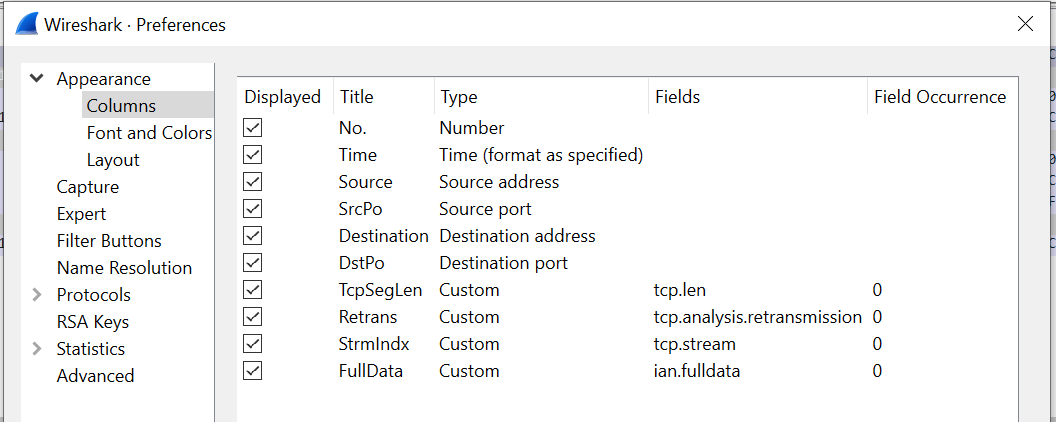
The Stream Index (tcp.stream), conveniently calculated for us by Wireshark, is a unique index that identifies the 5-tupple of the IP address, port pairs, and protocol1. This is going to be critical later in restricting the complexity of the message matching, but we’ll come to that.
I’m also exporting Retransmission (tcp.analysis.retransmission) as, whilst I’m not using it currently, it might come in handy in the future analysis of any delayed responses.
Finally, I’m also exporting the full, unexpurgated, data, captured in the ian.fulldata field. We only capture 50 bytes of the TCP payload here, so that’s not a problem, but caveat emptor if you choose to do the same with more.
As mentioned above, this seems to require a specialised Lua dissector, which is not difficult, and shown below. This code simply registers a post-dissector routine (one that runs when everything else has done its work) and adds the full data from the tcp.payload as hex pairs to a new field.
-- define a protocol

datapost = Proto("datapost", "Ian")

-- Create a field extractor for the payload

tcp_payload_f = Field.new("tcp.payload")

local string_field = ProtoField.string("ian.fulldata", "Full data")

datapost.fields = { string_field, }

function datapost.dissector(tvb, pinfo, tree) local subtree = tree:add(datapost)

    -- Extract all values for this field

    local tcp_payload_ex = tcp_payload_f()

    if tcp_payload_ex then
        subtree:add( string_field, tostring(tcp_payload_ex.range:bytes()) )
    end
end

register_postdissector(datapost)
Reading the CSV
The capture here is of some 16.1 million datagrams. The PCAP file is 1.6 GB, and the exported CSV, even with the limited fields selected, 2.65 GB uncompressed. The file can be read either by the readr::read_csv() routine used previously, which returns a tibble, or the faster data.table::fread() routine, as discussed above. In any event the stripped down file doesn’t take too long to load in either, but the later is most definitely preferred during development when the full data output is being used:
| Routine | Time | Time (full data) |
|---|---|---|
| readr::read_csv() | 134 seconds | 770 seconds |
| data.table::fread() | 29 seconds2 | 64 seconds |
fread() also has the advantage that it can directly read 64 bit integers, unlike read_csv() which required us to read them as characters then convert afterwards. It also handles the flag fields slightly differently, so the post-read mutate clean-up needs to change slightly3:
# In addition to the previous article, this article is also going to require
# the following packages to be installed and loaded:

install.packages("data.table")
install.packages("R.utils")  # for DT to read gz files
install.packages("RSQLite")

library("data.table")
library("DBI")

# Read and lightly massage the data

pcapData =
fread(  csvFile1,
        colClasses = list( integer = c( "No.",
                                        "SrcPo",
                                        "DstPo",
                                        "TcpSegLen"
                                       ),
                           character  = c( "Time",
                                           "Source",
                                           "Destination",
                                           "Retrans",
                                           "StrmIndx",
                                           "FullData"
                                           )
                           )
        ) %>%
mutate( Retrans = if_else( Retrans == "", NA, TRUE ) )
Data preparation is straightforward. We simply filter out all messages without a TCP payload, flag input messages, then examine the FullData fields exported by our Lua dissector with grepl() to see which contain the input message we want to analyse. We flag these, too.
Whilst we’re here, we’ll also convert the time to a numeric seconds value. (Somewhat confusingly, this variable displays in RStudio as an integer, but closer examination shows it contains fractional digits which retain its original microsecond precision.)
pcapData <-
  pcapData %>%
  filter( !(TcpSegLen == 0 | is.na(TcpSegLen)) ) %>%
  mutate( ToTpf = if_else( Destination %in% TpfIps, TRUE, FALSE ) ) %>%
  mutate( `w$tkd` = grepl("E65BE3D2C4", FullData),    # "W$TKD"
          # get time in seconds (shows as secs but has us resolution)
          secs = as.numeric(strptime(Time, "%Y-%m-%d %H:%M:%OS", tz=""))
          )
Now we need to pair up the response with the input message. As this protocol is a simple request/response, this is straightforward: ignoring retransmissions, the first datagram after a flagged input message is considered to be the response (the response may be in multiple datagrams). Clearly we have to consider only responses which have the same ip address and port pairs as the request, for which we’ll use Wireshark’s Stream Index 5-tuple, discussed earlier. To ensure we don’t waste excessive resources looking too far into the future, we’ll limit our examination window to 30 seconds from the time of the input message.
A number of methods for performing this matching were tried out, but by far the fastest was to use the RSQLite package to create an SQLite database and use SQL to perform the matching. An in-memory database would probably be sufficient for this task, if you have enough RAM, though adequate speed was obtained using one SSD-based.
In order to speed up the matching only the bare minimum of columns for a single stream of data was loaded into the database at any one time. An index was created on the message flag column as an explain query plan suggested that it would use one. The SQL query then returned the options, selected the first for each input, and calculated the elapsed time.
The results are then recombined with the full data row, the input and output messages extracted and converted from EBCDIC, and the LNIATAs extracted and verified as matching.4
pairupTxs <- function(df) {
  mydb <- dbConnect( RSQLite::SQLite(), dbName )
    dbWriteTable( mydb, "ipTrace", overwrite = TRUE,
                  df %>% select( `No.`, secs, ToTpf, `w$tkd` )
                  )

    dbExecute( mydb, "create index ixtkd on ipTrace(`w$tkd`)" )

    sqlCmd <- glue("select trin.`No.` InNo,
                       min(trout.`No.`) OutNo, (trout.secs-trin.secs)*1000 Response
               from ipTrace trin
               join ipTrace trout
               on
                  trin.`w$tkd` = 1 and
                  trin.`No.` < trout.`No.` and
                  trout.secs < (trin.secs+30)
               group by trin.`No.`")

    queryResults <- dbGetQuery( mydb, sqlCmd )

  dbDisconnect(mydb)

  results =
    queryResults %>%
    left_join( df, by=c("InNo"="No.") ) %>%
    left_join( df %>% select( `No.`, FullData) ,
               by=c("OutNo"="No.")
               ) %>%
    rename( FullData.In = FullData.x,
            FullData.Out = FullData.y
            ) %>%
    mutate( lniata.In  = stringr::str_sub(FullData.In, 27, 38),
            lniata.Out = stringr::str_sub(FullData.Out, 21, 32),
            message.In  = stringr::str_sub(FullData.In, 61),
            message.Out = stringr::str_sub(FullData.Out, 45)
            ) %>%
    mutate( message.In  = purrr::map( message.In,  ~convertEbcdic(.x) ),
            message.Out = purrr::map( message.Out, ~convertEbcdic(.x) ),
            lniata.Mismatch = (lniata.In != lniata.Out)
            )
  return(results)
}

pairedResults <-
  pcapData %>%
  mutate(si2 = StrmIndx) %>%
  group_by( si2 ) %>%
    group_modify( ~ pairupTxs(.x) ) %>%
  ungroup() %>%
  select( - si2 )
Presentation of results
It is now a simple matter of running some summary statistics on the response times. I chose to report the following:
- Transaction count
- Median
- Median Absolute Deviation
- Minimum
- Maximum
- 90th percentile
- 99th percentile
These values are easily obtained:
countResponse = length( pairedResults$Response )
medianResponse = median( pairedResults$Response )
madResponse = mad( pairedResults$Response )
minResponse = min( pairedResults$Response )
maxResponse = max( pairedResults$Response )
q90Response = quantile( pairedResults$Response, 0.90 )[[1]]
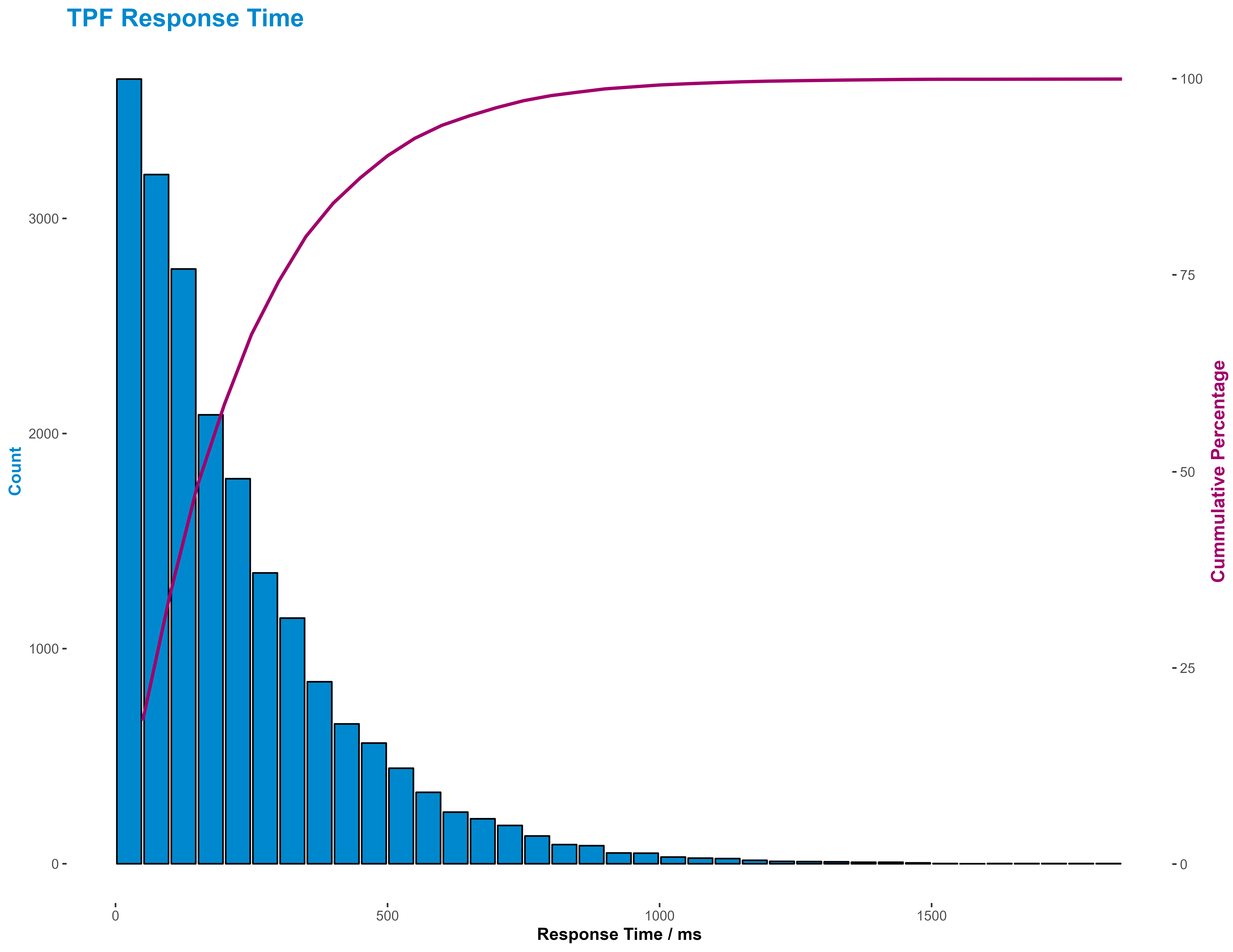
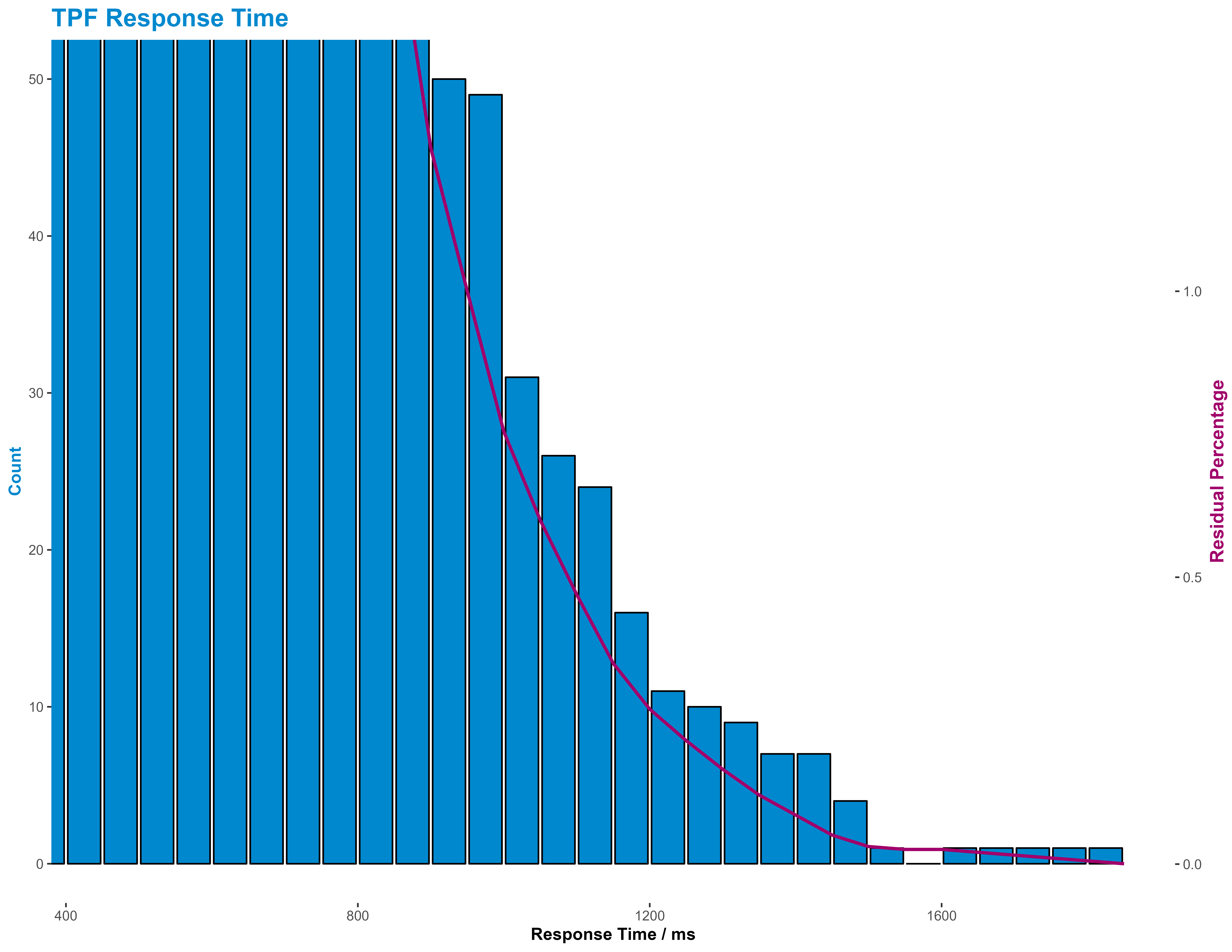
q99Response = quantile( pairedResults$Response, 0.99 )[[1]]But, as with most summary statistics, they don’t really give a good idea of the distribution of response times. This is probably best done either using a cumulative distribution function line graph or a histogram. I favoured the later here as being easier to interpret, though I supplemented it with a cumulative percentage line.
I also presented the tail of the response time, as that’s where our real interest lies, in the same way, but this time using a residual percentage line.
R Note: I usually use cut() to bin data, but hist() returns low and mid values as well, which are useful when plotting.
histResponses <- hist( pairedResults$Response, breaks=40, plot=FALSE )
histResponses <-
  with( histResponses,
        tibble( count = c(counts, NA),
                low = breaks,
                mid = c(mids, NA)
                )
        ) %>%
  mutate( high = dplyr::lead(low, 1),
          cumPerc = 100* cumsum(count) / sum(count, na.rm=TRUE),
          resPerc = 100 - cumPerc
          ) %>%
  head( -1 )

maxX = max( histResponses$high )
maxY1 = max(histResponses$count, na.rm=TRUE)
maxY2 = 100

y2Coeff = maxY2/maxY1

# Use corporate colours!

sncfBlue = "#0088CE"
sncfPrune = "#a1006b"
sncfVertPomme = "#82be00"

# Build common base plot

histPlotBase <-
  ggplot( histResponses ) +
    geom_bar( aes( x = mid,   # x is the mid-bin bucket
                   y = count
                   ),
              stat = "identity",
              color = "#000000",
              fill = sncfBlue
              ) +
    labs(
      title = "TPF Response Time",
      caption = "Source: TPF IP Trace",
      x = "Response Time / ms",
      y = "Count"
    ) +
    theme_classic() +
    theme(
      legend.background = element_blank(),
      legend.key = element_blank(),
      panel.background = element_blank(),
      panel.border = element_blank(),
      strip.background = element_blank(),
      plot.background = element_blank(),
      axis.line = element_blank(),
      panel.grid = element_blank(),
      plot.title = element_text(color = sncfBlue, size = 16, face = "bold"),
      plot.subtitle = element_text(size = 10, face = "bold"),
      plot.caption = element_text(face = "italic"),
      axis.title.x = element_text(  face = "bold"),
      axis.title.y.left  = element_text( angle = 90,
                                         color = sncfBlue,
                                         face = "bold"
                                         ),
      axis.title.y.right = element_text( angle = 90,
                                         color = sncfPrune,
                                         face = "bold",
                                         size=12
                                         )
      )

# Customise for overview

histPlot1 = histPlotBase +
  scale_y_continuous(
      sec.axis = sec_axis( ~ . * y2Coeff,
                           name = "Cummulative Percentage"
                           )
      ) +
  geom_line( aes( x = high,  # x here is the vale at the high end of the bucket
                  y = cumPerc / y2Coeff
                  ),
             color = sncfPrune,
             size = 1
             )

# Customise for tail view

histPlot2 = histPlotBase +
  coord_cartesian( xlim = c(450, maxX),
                   ylim = c(0, 50)
                   ) +
  scale_y_continuous(
      sec.axis = sec_axis( ~ . * y2Coeff,
                           name = "Residual Percentage"
                           )
      ) +
  geom_line( aes( x = high,
                  y = resPerc / y2Coeff
                  ),
             color = sncfPrune,
             size = 1
             )
To respect customer confidentiality, I’m not going to show the actual results, but to see what the general output of the histograms look like we can generate some response times using a simple gamma function:
pairedResults = tibble( Response = rgamma( 20000, 1.1, 0.05 ) * 10 )and plot those instead:
Summary
We have seen in this both this article, and the preceding one, how we might use the Wireshark application in conjunction with R scripts to convert and analyse large volumes of IP trace traffic captured on an IBM z/TPF, or other, system, particularly one without an interactive IP trace explorer dashboard, and present that in a fashion that is easy to share our problem investigations graphically with our business partners, but also quick to reprogram to extract specific information that they may request.
This article extends our previous analysis to match requests and responses and generate a distribution of response time for our system.
Thanks
This article is based on work performed for SNCF, and is published with their permission, for which many thanks.
Footnotes
It may also uniquely identify a conversation, that is an exchange of datagrams bracketed by SYN/FIN exchanges, but I haven’t been able to confirm this.↩︎
fread() actually self-reports its elapsed time to be 19 seconds but, for consistancy, times were measured by a surrounding tictoc pair. The difference is suspected to possibly be garbage collection.↩︎
Errata: Here, StrmIndex is read in as a character field. This is unnecessary. It’s probably better to treat it as an integer.↩︎
There are a couple of oddities here. Firstly, if you think the convertEbcdic routine looks like a terrible hack, then I’d have to agree with you. Getting this working was rather more difficult than expected and I didn’t have the time to improve it. As Blaise Pascal wrote, “Je n’ai fait celle-ci plus longue que parce que je n’ai pas eu le loisir de la faire plus courte.” (I have made this longer than usual because I have not had time to make it shorter) -- “Lettres Provinciales” (1657). Secondly, the code to build pairedResults builds a copy of StrmIndx in si2. This would seem unnecessary and I’m, as yet, unable to account for why group_by() refused to accept the former as its argument.↩︎